Learning Bayesian Hierarchical Modeling from 8 Schools
The problem we’re discussing in this post appears in Bayesian Data Analysis, 3rd edition (Gelman et al., 2013). Here, Gelman et al. describe the results of independent experiments to determine the effects of special coaching programs on SAT scores.
There are \(J = 8\) schools in this experiment. For the \(j\)th experiment \(j = 1,\dots,J\), one observes an estimated coaching effect \(y_j\) with associated standard error \(\sigma_j\), the values of the effects and standard errors are displayed in the table below. We only observe \(\mathbf{y}=\{y_1,\dots,y_n\}\) and \(\boldsymbol{\sigma}=\{\sigma_1,\dots,\sigma_j\}\), instead of the original full dataset.
| A | 28 | 15 |
| B | 8 | 10 |
| C | -3 | 16 |
| D | 7 | 11 |
| E | -1 | 9 |
| F | 1 | 11 |
| G | 18 | 10 |
| H | 12 | 18 |
From BDA3, we consider that the estimates \(y_j\) are obtained by independent experiments and have approximately normal sampling distributions with known sampling variances, as the sample sizes in all of the eight experiments were relatively large, with over thirty students in each school.
Non-Hierarchical Methods
Separate estimates
From the table above, we might suspect that schools tend to have different coaching effects – some schools have rather high estimates (like schools A and G), some have small effects (like schools D and F), and some even have negative effects (schools C and E). But the problem is that the standard errors of these estimated effects are very high. If we treat each school as individual experiments and apply separate normal distributions with these values, we see that all of their 95% posterior intervals overlap substantially.
y <- c(28, 8, -3, 7, -1, 1, 18, 12)
sigma <- c(15, 10, 16, 11, 9, 11, 10, 18)

q_025 <- rep(0, 8)
q_975 <- rep(0, 8)

for (i in 1:8){
    q_025[i] <- qnorm(0.025, mean = y[i], sd = sigma[i])
    q_975[i] <- qnorm(0.975, mean = y[i], sd = sigma[i])
}

print(cbind(y, sigma, q_025, q_975))
      y sigma     q_025    q_975
[1,] 28    15  -1.39946 57.39946
[2,]  8    10 -11.59964 27.59964
[3,] -3    16 -34.35942 28.35942
[4,]  7    11 -14.55960 28.55960
[5,] -1     9 -18.63968 16.63968
[6,]  1    11 -20.55960 22.55960
[7,] 18    10  -1.59964 37.59964
[8,] 12    18 -23.27935 47.27935
Pooled estimates
The above overlap based on independent analyses seems to suggests that all experiments might be estimating the same quantity. We can take another approach, and that is to treat the given data as eight random sample under a common normal distribution with known variances. With a noninformative prior, it can be shown that the posterior mean and variance is the inverse weighted average of \(\mathbf{y}\).
\[\bar{y} = \frac{\sum_j\frac{y_j}{\sigma_j^2}}{\sum_j \frac{1}{\sigma_j^2}}, \quad \text{Var}(\bar y)=\frac{1}{\sum_j \frac{1}{\sigma_j^2}}\]cat(paste('Posterior mean:', sum(y/sigma^2)/sum(1/sigma^2)), '\n')
cat(paste('Posterior variance:'), 1/sum(1/sigma^2))
Posterior mean: 7.68561672495604
Posterior variance: 16.58053
The \(\chi^2\) test for the hypothesis that the estimates are sampled from a common normal distribution yields that a very high p-value, which supports the notion that they are indeed from the same distribution. However, Gelman et al also argues that
“The pooled model implies the following statement: ‘the probability is 0.5 that the true effect in A is less than 7.7,’ which, despite the non-significant \(\chi^2\) test, seems an inaccurate summary of our knowledge. The pooled model also implies the statement: ‘the probability is 0.5 that the true effect in A is less than the true effect in C,’ which also is difficult to justify given the data…”
Ideally, we want to combine information from all of these eight experiments without assuming the \(y_j\)’s are observations of under a common distribution. Let’s turn our attention to a hierarchical setup.
Bayesian Hierarchical Modeling
We can model this dataset as such: the coaching effect \(y_j\) is normally distributed with mean \(\theta_j\) and known variance \(\sigma_j^2\) , independently across \(j=1,\dots,J\). \(\theta_1,\dots,\theta_J\) are drawn independently from a normal population with mean \(\mu\) and variance \(\tau^2\). This also allows for the interpretation of each \(\theta_j\)’s (the true coaching effect of each school) as a random sample from a shared distribution (say, the coaching quality of a school in a particular geographical region).
The vector of parameters \((\mu,\tau)\) is assigned a noninformative uniform prior \(p(\mu,\tau)\propto 1\).
With this setup, we can try to combine the coaching estimates in some way to obtain improved estimates of the true effects \(\theta_j\).
We can write an expression for the unnormalized full posterior density \(p(\boldsymbol{\theta},\mu,\tau \vert \mathbf{y},\boldsymbol{\sigma})\):
\[\begin{aligned} p(\boldsymbol{\theta},\mu,\tau|\mathbf{y},\boldsymbol{\sigma}) &\propto p(\boldsymbol{\theta}|\mu,\tau)\times p(\mu,\tau)\times p(\mathbf{y}|\boldsymbol{\theta},\boldsymbol{\sigma}) \cr &\propto \prod_{j=1}^J p(\theta_j|\mu,\tau)p(y_j|\theta_j,\sigma_j) \cr &\propto \prod_{j=1}^J \left(\frac{1}{\tau\sqrt{2\pi}}\exp\left(-\frac{(\theta_j-\mu)^2}{2\tau^2}\right)\frac{1}{\sigma_j\sqrt{2\pi}}\exp\left(-\frac{(y_j-\theta_j)^2}{2\sigma_j^2}\right)\right) \cr &\propto \prod_{j=1}^J \left(\frac{1}{\tau\sigma_j}\exp\left(-\frac{(\theta_j-\mu)^2}{2\tau^2}-\frac{(y_j-\theta_j)^2}{2\sigma_j^2}\right)\right) \end{aligned}\]Next, we can decompose the full posterior density into the conditional posterior, \(\theta_j\vert\mu,\tau,y,\sigma\), and marginal posterior, \(p(\mu,\tau\vert\mathbf{y},\boldsymbol{\sigma})\), both of which are a product of \(J\) independent components. Also note that
\[\frac{1}{\sigma_j^2}+\frac{1}{\tau^2}=\frac{\tau^2+\sigma_j^2}{\sigma_j^2\tau^2}\implies \sigma_j\tau=\sqrt{\frac{\tau^2+\sigma_j^2}{\frac{1}{\sigma_j^2}+\frac{1}{\tau^2}}}\]which will be useful in matching the variance part of the normal densities in this decomposition.
\[\begin{aligned} p(\theta,\mu,\tau|y,\sigma) &\propto \prod_{j=1}^J \frac{1}{\tau\sigma_j}\exp\left\{-\frac{1}{2}\left(\frac{(\theta_j-\mu)^2}{\tau^2}+\frac{(y_j-\theta_j)^2}{\sigma_j^2}\right)\right\} \cr &\propto \prod_{j=1}^J\frac{1}{\tau\sigma_j}\exp\left\{-\frac{1}{2}\left(\frac{\sigma_j^2(\theta_j-\mu)^2+\tau^2(y_j-\theta_j)^2}{\tau^2\sigma_j^2}\right)\right\} \cr &\propto \prod_{j=1}^J\frac{1}{\tau\sigma_j}\exp\left\{-\frac{1}{2}\left(\frac{\sigma_j^2(\theta_j^2-2\mu\theta_j+\mu^2)+\tau^2(y_j^2-2y_j\theta_j+\theta_j^2)}{\tau^2\sigma_j^2}\right)\right\} \cr &\propto \prod_{j=1}^J\frac{1}{\tau\sigma_j}\exp\left\{-\frac{1}{2}\left(\frac{\theta_j^2(\sigma_j^2+\tau^2)-2\theta_j(\mu\sigma_j^2+y_j^2)+\sigma_j^2\mu^2+\tau^2y_j^2}{\tau^2\sigma_j^2}\right)\right\} && \text{(quadratic expression in terms of $\theta_j$)} \cr &\propto \prod_{j=1}^J\frac{1}{\tau\sigma_j}\exp\left\{-\frac{1}{2}\left(\frac{(\sigma_j^2+\tau^2)\left[\theta_j-\frac{\mu\sigma_j^2+y_j\tau^2}{\sigma_j^2+\tau^2}\right]^2-\frac{(\mu\sigma_j^2+y_j\tau^2)^2}{\sigma_j^2+\tau^2}+\sigma_j^2\mu^2+\tau^2y_j^2}{\tau^2\sigma_j^2}\right)\right\} && \text{(completing the square)} \cr &\propto \prod_{j=1}^J \sqrt{\frac{\frac{1}{\sigma_j^2}+\frac{1}{\tau^2}}{\tau^2+\sigma_j^2}} \exp\left\{-\frac{1}{2}\left(\frac{1}{\sigma_j^2}+\frac{1}{\tau^2}\right)\left[\theta_j-\frac{\mu/\tau^2+y_j/\sigma_j^2}{1/\tau^2+1/\sigma^2}\right]^2 \right. \cr &\mathrel{\phantom{=}} \left. -\frac{1}{2\tau^2\sigma_j^2}\times\frac{\bcancel{-\mu^2\sigma_j^4}-2\mu\sigma_j^2y_j\tau^2\bcancel{-y_j^2\tau^4}+\bcancel{\sigma_j^4\mu^4}+\sigma_j^2\mu^2\tau^2+\tau^2y_j^2\sigma_j^2+\bcancel{\tau^4y_j^2}}{\sigma_j^2+\tau^2}\right\} \cr &\propto \prod_{j=1}^J \sqrt{\frac{1}{\sigma_j^2}+\frac{1}{\tau^2}} \exp\left\{-\frac{1}{2}\left(\frac{1}{\sigma_j^2}+\frac{1}{\tau^2}\right)\left[\theta_j-\frac{\mu/\tau^2+y_j/\sigma_j^2}{1/\tau^2+1/\sigma^2}\right]^2\right\} \cr &\quad \times \frac{1}{\sqrt{\tau^2+\sigma_j^2}} \exp\left\{-\frac{1}{2}\frac{(\mu-y_j)^2}{\sigma_j^2+\tau^2}\right\} \cr &\propto \prod_{j=1}^J \theta_j|\mu,\tau,y,\sigma \sim N(\hat\theta_j,V_j) \times \phi\left(y_j|\mu,\sqrt{\sigma_j^2+\tau^2}\right) \end{aligned}\]where
\[\hat\theta_j=\frac{\frac{y_j}{\sigma_j^2}+\frac{\mu}{\tau^2}}{\frac{1}{\sigma_j^2}+\frac{1}{\tau^2}},\quad V_j=\frac{1}{\frac{1}{\sigma_j^2}+\frac{1}{\tau^2}}\]and \(\phi(y\vert\mu,\sigma)\) denotes the normal density with mean \(\mu\) and standard deviation \(\sigma\).
By forming a quadratic expression in terms of \(\theta_j\) and completing the square, we have now decomposed the posterior into two key constituents, both of which are also normal distributions. The first term in the product is the conditional posterior – the distribution of the true coaching effect conditioned on latent parameters \(\mu\), \(\tau\), and the data. The second term is the marginal posterior, which describes the distribution of the observed data given values of \(\mu\) and \(\tau\).
The posterior mean, \(\hat\theta_j\), is a precision-weighted average of the prior population mean and the sample mean of the $j$-th group; these expressions for \(\hat{\theta}_j\) and \(V_j\) are functions of \(\mu\) and \(\tau\) as well as the data. In other words, the posterior distribution offers a compromise between our prior beliefs and the observed data.
Parameter Estimation
The solution is not yet complete, because \(\mu\) and \(\tau\) are still unknown. For this hierarchical model, we can make use of the marginal posterior we have derived earlier since estimates of the true effect can be calculated from \(\mu\), \(\tau\) and the given data.
Consider a transformed set of parameters \((\lambda_1, \lambda_2)\), where \(\lambda_1=\mu\) and \(\lambda_2=\log\tau\). In Bayesian inference, transformation of parameters is useful for reducing skewness of the posterior distribution or for ease of simulation. For example, in the marginal posterior density, only positive values of \(\tau\) are meaningful, so it would be desirable to transform this parameter to the real line. Recall that the change-of-variable formula: in the univariate case, if the pdf of random variable \(X\) is \(f_X(x)\) and \(Y=g(X)\) where \(g\) is a bijective and differentiable function, the pdf of \(y\) is given by
\[f_Y(y) = f_X(x)\vert J\vert,\quad \text{where } J=\frac{\mathrm{d}x}{\mathrm{d}y}, \quad x=g^{-1}(y)\]We can try to get a good estimate of \((\lambda_1,\lambda_2)\) by finding the set of values in which the posterior is maximized. This is equivalent to maximizing the log of the posterior, which helps avoid exceeding the precision of floating point numbers due to potentially massive number of multiplication operations involved.
Now we can write the log posterior as
\[\log p(\lambda_1,\lambda_2\vert \mathbf{y},\boldsymbol{\sigma}) \propto \sum_{j=1}^J \left[-\frac{1}{2}\log\left(\exp\left\{2\lambda_2\right\}+\sigma_j^2\right) - \frac{(\lambda_1-y_j)^2}{2(\sigma_j^2+\exp\left\{2\lambda_2\right\})}\right]+\lambda_2\]where the last term comes from the Jacobian.
Let’s visualize the log posterior with a contour plot.
# given data
y <- c(28, 8, -3, 7, -1, 1, 18, 12)
sigma <- c(15, 10, 16, 11, 9, 11, 10, 18)

# defining the log posterior for lambda
logpost <- function(lambda, sigma, y){
  sum(-0.5*log(exp(2*lambda[2])+sigma^2) -
        ((lambda[1]-y)^2)/(2*(sigma^2+exp(2*lambda[2])))) +
        lambda[2]
}

# grids
lambda_1 <- seq(from = -18, to = 37, by = 0.1)
lambda_2 <- seq(from = -6, to = 4.1, by = 0.1)
z <- matrix(0, nrow = length(lambda_1), ncol = length(lambda_2))

for (i in 1:length(lambda_1)){
  for (j in 1:length(lambda_2)){
    lambda <- c(lambda_1[i], lambda_2[j])
    z[i,j] <- logpost(lambda, sigma, y)
  }
}

contour(x = lambda_1, y = lambda_2, z = z, col = "blue", nlevels = 40,
        xlab = expression(lambda[1]), ylab = expression(lambda[2]),
        cex.axis = 1.1, cex.lab = 1.3)
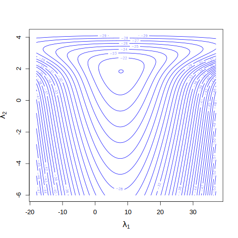
From the contour plot, the mode seems close to \((8,2)\). We shall use this as a starting guess in optim() to find the posterior mode and covariance matrix by approximating the log posterior to a (multivariate) normal distribution.
out <- optim(par = c(8, 2), fn = logpost, control = list(fnscale = -1),
            hessian = TRUE, sigma = sigma, y = y)
cat('Posterior mode:\n')
print((post_mode <- out$par))
cat('\n')
cat('Covariance matrix: \n')
print((post_cov <- -solve(out$hessian)))
Posterior mode:
[1] 7.926685 1.841525

Covariance matrix:
          [,1]      [,2]
[1,] 22.3232882 0.1935228
[2,]  0.1935228 0.5352576
The normal approximation to the posterior of \((\lambda_1,\lambda_2)\) is \(\lambda_1,\lambda_2\vert\sigma,y\sim N\left( \begin{bmatrix} 7.926685 \cr 1.841525 \end{bmatrix}, \begin{bmatrix} 22.3232882 & 0.1935228 \cr 0.1935228 & 0.5352576 \end{bmatrix} \right)\)
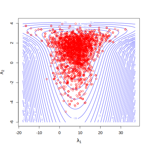
The covariance matrix will be useful when sampling for values of \((\lambda_1, \lambda_2)\) using MCMC methods later. Although we can sample values from this normal approximation, it would not be as accurate as sampling from the log posterior itself. To do that, we can use the Metropolis-Hastings algorithm.
MCMC Sampling
The Metropolis-Hastings (MH) algorithm is a MCMC method to generate random samples from a density where direct sampling might be difficult (e.g. where normalizing constants are intractable or for high dimensional densities). As this post gets rather lengthy, I shall skip the introduction to the MH algorithm or reserve it for future posts.
Here, we will use MH algorithm to draw 10000 samples. We will use our normal approximation density has the proposal here, as it is the closest to our target posterior density and hence it is more likely to generate accepted samples. The first 5000 samples will be treated as burn-in and discarded; desired samples are obtained after the stationary distribution is reached.
library(LearnBayes)
library(coda)

set.seed(11)

iters <- 10^4
proposal <- list(var = post_cov, scale = 2)

# random walk metropolis
fit1 <- rwmetrop(logpost, proposal, start = post_mode, iters, sigma, y)

# overlaying last 5000 draws on contour plot of the log posterior
contour(x = lambda_1, y = lambda_2, z = z, col = "blue", nlevels = 40,
        xlab = expression(lambda[1]), ylab = expression(lambda[2]),
        cex.axis = 1.1, cex.lab = 1.3)
points(x = fit1$par[5001:iters,1], y = fit1$par[5001:iters,2], col = "red")
cat('Acceptance rate: \n')
print(fit1$accept)
Acceptance rate:
[1] 0.3288
par(mfrow=c(2,1))
plot(density(fit1$par[5001:iters,1]), main = "", xlab = expression(lambda[1]))
plot(density(fit1$par[5001:iters,2]), main = "", xlab = expression(lambda[2]))
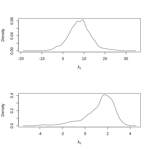
The sampling acceptance rate is 32.88%, which is reasonable, and we observe that the MCMC samples \(\lambda_1\) and \(\lambda_2\) approximate unimodal distributions with modes near the values of the posterior modes found earlier. Next, we perform an MCMC output analysis to study convergence of this Markov chain.
mcmcobj1 <- mcmc(fit1$par[5001:iters,])
colnames(mcmcobj1) <- c("lambda_1", "lambda_2")
par(mfrow=c(2,1))
traceplot(mcmcobj1)
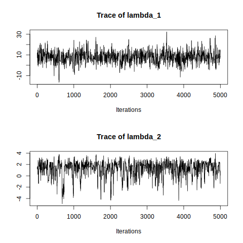
The traceplots of both \(\lambda_1\) and \(\lambda_2\) resemble random noise, generally showing great flunctuation. This suggests that the samples of both \(\lambda_1\) and \(\lambda_2\) do not have high serial correlation/dependence and has mixed well.
It is also important to analyze the degree of autocorrelation in the sampled values. In an MCMC algorithm like the random-walk Metropolis-Hastings above, the simulated value of \(\theta\) at \((t+1)\)th iteration is dependent on the simulated value at the $t$th iteration. If strong correlation is detected, we can say that two consecutive samples provide only marginally more information about the posterior distribution than a single simulated draw. It might also prevent the algorithm from sufficiently exploring the parameter space.
par(mfrow=c(2,1))
autocorr.plot(mcmcobj1, auto.layout = FALSE)
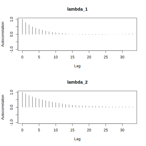
Here, the autocorrelation plots show fast decay in both \(\lambda_1\) and \(\lambda_2\); autocorrelations are close to 1 for lag one but reduce quickly as a function of lag, indicating a low degree of autocorrelation.
With a satisfactory MCMC output analysis, we can use these samples to obtain samples of true effects, \(\theta_j\). For each school, we map every pair of sampled \((\lambda_1, \lambda_2)\) back to a pair of \((\mu,\tau)\). Recall that \(\theta_j\vert\mu,\tau,y,\sigma \sim N(\hat\theta_j,V_j)\) where \(\hat\theta_j\) and \(V_j\) are functions of \(\mu\) and \(\tau\), thus we will use each of the 5000 pairs of \((\mu,\tau)\) as parameters to a normal distribution to generate a sample of \(\theta_i\).
# the last 5000 MCMC samples (lambda_1, lambda_2)
lambda_samples <- fit1$par[5001:iters,]

# function to compute mean
theta_hat <- function(lambda, y_j, sigma_j){
    ((y_j/sigma_j^2)+(lambda[,1]/exp(2*lambda[,2]))) /
    ((1/sigma_j^2)+(1/exp(2*lambda[,2])))
}

# function to compute variance
V <- function(lambda, y_j, sigma_j){
    1 / (1/sigma_j^2 + 1/exp(2*lambda[,2]))
}

# drawing 5000 samples of theta_j
theta_samples <- function(lambda, y_j, sigma_j){
    rnorm(5000, mean = theta_hat(lambda, y_j, sigma_j),
          sd = sqrt(V(lambda, y_j, sigma_j)))
}

theta_mean <- rep(0, 8)
theta_sd <- rep(0,8)

# the joint posterior density of (theta_1,...,theta_j)
theta_all <- matrix(0, nrow = 5000, 8)
    for (j in 1:8){
        thetas <- theta_samples(lambda_samples, y[j], sigma[j])
        theta_all[,j] <- thetas
        theta_mean[j] <- mean(thetas)
        theta_sd[j] <- sd(thetas)
}

print(theta_dist <- cbind(theta_mean, theta_sd))
     theta_mean theta_sd
[1,]  11.226786 8.510583
[2,]   7.812253 6.185383
[3,]   6.078697 7.993831
[4,]   7.609353 6.515474
[5,]   5.162853 6.381664
[6,]   6.231208 6.729192
[7,]  10.340858 6.990141
[8,]   8.490497 8.045273
We arrive at estimates of the true coaching effect \(\theta_j\)’s from our hierarchical model. The differences between schools are not as drastic as $y_j$’s, and this is related to the concept of shrinkage.
Shrinkage
From the conditional posteriors above, we can find that the posterior mean of \(\theta_j\), conditioned on \((\mu,\tau)\), can be written as
\[\mathrm{E}(\theta_j\vert\mu,\tau,\mathbf{y},\boldsymbol{\sigma}) = (1-B_j)y_j + B_j\mu\]where
\[B_j = \frac{\tau^{-2}}{\tau^{-2}+\sigma^{-2}}\]is the size of the shrinkage of \(y_j\) towards \(\mu\). From the MCMC samples, we can calculate the shrinkage size for the treatment effect of each school.
# shrinkage function for each j
shrink_j <- function(lambda, sigma_j){
    (1/exp(lambda[,2]))^2 / ((1/exp(lambda[,2]))^2+1/sigma_j^2)
}

shrink <-rep(0, 8)

for(j in 1:8){
    shrink[j] <- mean(shrink_j(lambda_samples, sigma[j]))
}

print(data.frame(school = LETTERS[c(1:8)],
                 shrink_size = shrink,
                 rank_shrink =rank(shrink),
                 rank_sigma = rank(sigma)))
  school shrink_size rank_shrink rank_sigma
1      A   0.8328975         6.0        6.0
2      B   0.7376910         2.5        2.5
3      C   0.8458181         7.0        7.0
4      D   0.7620532         4.5        4.5
5      E   0.7096051         1.0        1.0
6      F   0.7620532         4.5        4.5
7      G   0.7376910         2.5        2.5
8      H   0.8676774         8.0        8.0
We observe that shrinkage and sigma values for each school have the same rank. This is consistent with the shrinkage formula above; since the squared inverse of \(\sigma_j\) is in the denominator, \(B_j\) has a positive relationship with \(\sigma_j\). This also means that the conditional posterior mean for schools with higher standard errors will be shrunk more towards the global mean.
The samples also provide a way draw other related inferences, such as the probability of seeing an effect as large as 28 for school A, which works out to be a very low value.
sum(theta_all[,1] > 28) / length(theta_all[,1])
0.0468
Note the contrast with the “separate estimates” approach we discussed earlier, which would imply that this probability is 50%, which seems overly large especially given the data from other schools.
We can also ask for the probability that school A has a greater coaching effect than the rest of the schools.
prob <-c()

for(j in 2:8){
    prob[j] <-mean(sum(theta_all[,1] > theta_all[,j])) / nrow(theta_all)
}

print(data.frame(school = LETTERS[c(1:8)], probability = prob))
  school probability
1      A          NA
2      B      0.6346
3      C      0.6800
4      D      0.6382
5      E      0.7162
6      F      0.6804
7      G      0.5382
8      H      0.5994
The probability that school A’s coaching effect is greater than the other schools doesn’t seem that large, even though the original estimates \(y_j\)’s might suggest so (with some schools’ estimates even dipping below 0).
Conclusion
In summary, Bayesian hierarchical modeling gives us a way to calculate “true effect” sizes that is otherwise hard to obtain (we only have unbiased estimates and standard errors from our dataset). Arguably, the assumptions of both the “separate estimates” and “pooled estimates” approach don’t fully capture the state of our knowledge to be able to use them convincingly. But with the hierarchical model, we now have a “middle ground” of sorts, and it is also flexible enough to incorporate both empirical data and any prior beliefs we might have, both summarized by the posterior distribution. Finally, we can obtain samples using MCMC methods, from which we can perform inferences.
Credits
I learnt of this interesting problem as a piece of assignment from my Bayesian Statistics class, ST4234 in NUS, taught by Prof Li Cheng. I also referred to Bayesian Data Analysis, 3rd edition by Gelman et al for further context and some relevant statistical arguments.
Cover image: Jason Leung (Unsplash)
References
Enjoyed reading this article? More articles you might like to read next: